Predicting a number from infinitely many possible outputs
- How do get an algorithm to systematically choose the most appropriate line/curve/ or anything to fit to the data
- Two types
- Linear Regression
- Non-linear Regression
Linear Regression
Fitting a straight line into your data
How it works
- Steps
- Feed your training set to your supervised learning algorithm
- Your algorithm will produce some function
f: a model ftakes new input feature and produces an estimate/prediction- may or may not be the actual true value (the output variable/“target”) for the training example
- ex) If you’re helping the client to sell the house, the true price of the house is unknown until you sell it
- Representing
f- Univariate linear regression
- linear regression w/ 1 input variable
- Univariate linear regression
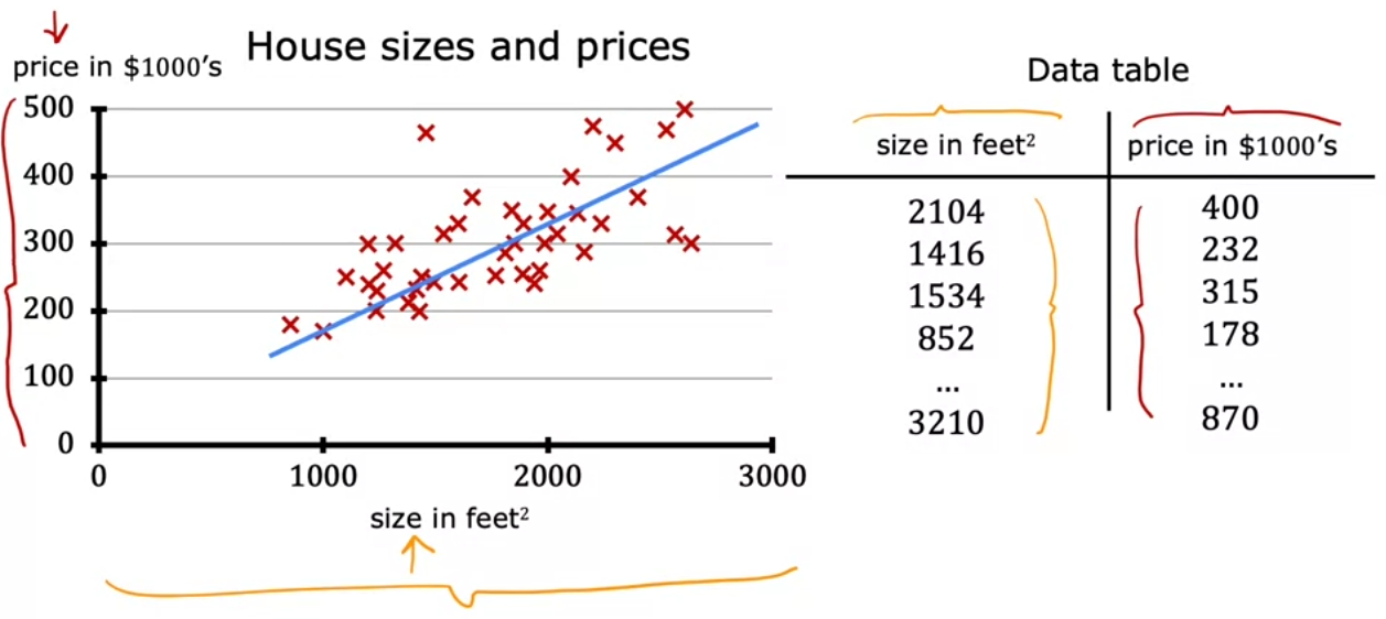
- Examples: Housing Price Prediction
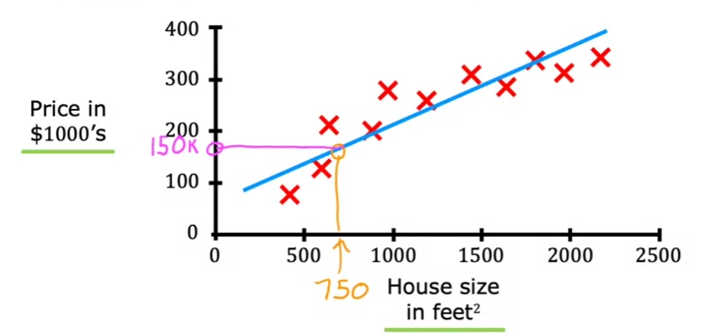
- This is a linear regression algorithm in supervised learning
- This algorithm fits a straight line. When your friends ask you the price for house size
750 ft^2, the algorithm gives you150k.
- This algorithm fits a straight line. When your friends ask you the price for house size
- This is a linear regression algorithm in supervised learning
- Another way to look at the data: tables!
More on Parameters
- The line “fits” differently based on and
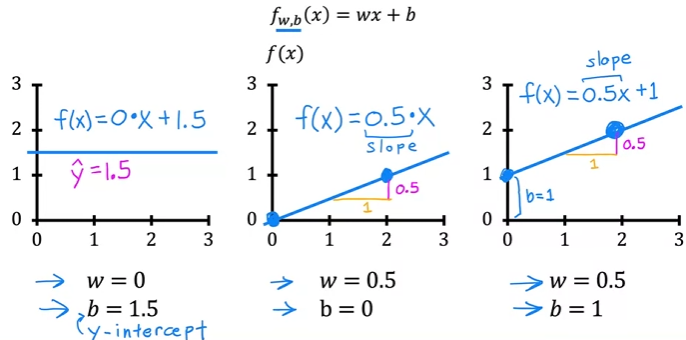
- The value of gives you the slope of the line
- How do you find values for and so that is close to for all ?
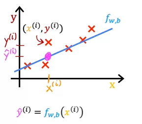
- There is a gap between and
- Use a cost function!
Cost function
Measures how well a line fits the training data
- Squared error cost function &=\frac{1}{2m}\sum_{i=1}^{m}(f_{w,b}(x^{(i)})-y^{(i)})^2 & \text{since } \hat{y}^{(i)}=f_{w,b}(x^{(i)}) \end{align}$$ - $m$ = the number of training examples - $\frac{1}{m}$ to get the *average* squared error - $\frac{1}{2m}$ for convention in ml - the most commonly used cost function for linear regression
- Mean absolute error (MAE)
- Mean squared error (MSE)
- Root mean squared error (RMSE)
- Linear regression tries to find values for and that makes as small as possible!
- Goal:
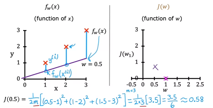
Visualization 1:
We will set to better understand intuitively
- function:
- parameter:
- cost function:
- goal:
- Example

- When then
- becomes a parameter in
- Example
- Example
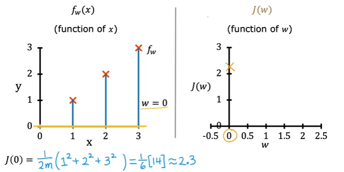
- For lots of different values for , you can get how the cost function looks like!
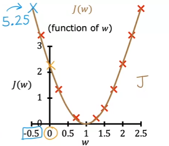
- Each value of corresponds to a different straight line fit
Visualization 2:
We will set to better understand intuitively
- function:
- parameter:
- cost function:
- goal:
- The fact that the cost function squares the loss ensures that the ‘error surface’ is convex like a soup bowl. It will always have a minimum that can be reached by following the gradient in all dimensions.
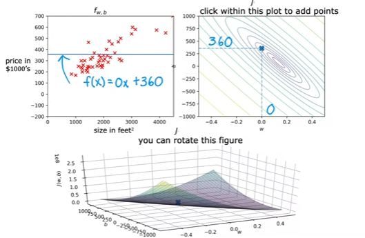
- The cost function visualization now:
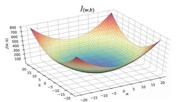
- Also curved under, except in 3 dimensions!
- It’s a 3D surface plot where the axes are labeled and
- As you vary the parameters in the cost function ( and ), you get different values in the surface function!
- You get the height
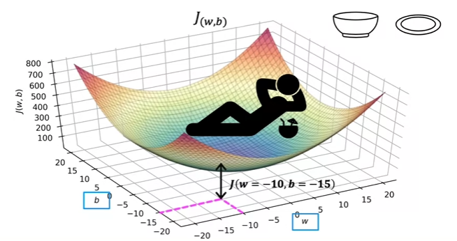
- You get the height
- Using contour plot
- A topological map shows high different mountains are. The contours are basically the horizontal slices of the mountain

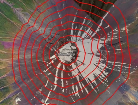
- Contour plot of the cost function
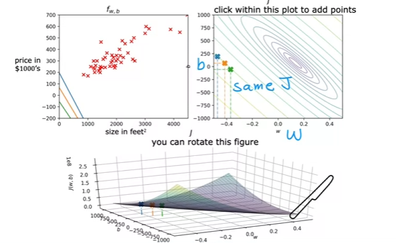
- Bottom
- The same bowl, just veeeeery stretched
- Up right - contour plot of cost function
- each axis is and
- each ovals (ellipses) shows the center points on the 3D surface which are at the exact same height, so the same value for
- You “slice” the 3D surface plot horizontally
- contour plots are convenient to visualize the 3D cost function
- Bottom
- A topological map shows high different mountains are. The contours are basically the horizontal slices of the mountain
- Examples
- Example
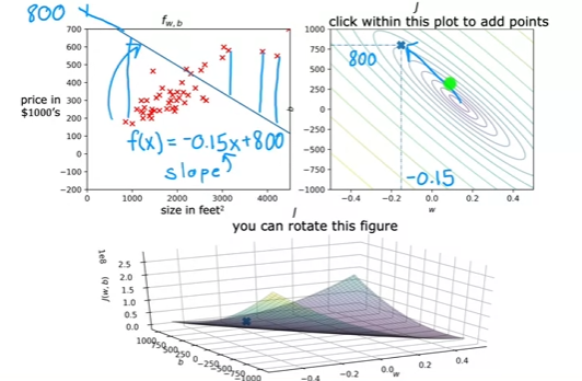
- You can see that the cost function value is far from the minima (the smallest circle)
- It’s generall not a good fit lol
- Example
- Example

- Manually looking at the contour map to find the best parameters is not recommended (also it will get more and more complex with complex algorithms)
- Instead write code that automatically finds the best parameter values
- Gradient descent!!!
- Example
Code (Google Colab)
Non-linear regression
Fitting a curve (more complex than straight line)