Vector in code (+ basic operations)

• https://colab.research.google.com/drive/1_1reeADTDwMw7ai4Ir27-v68tnUqCEy3?authuser=0#scrollTo=YS17ItgzdPpB
• Related: python list, NumPy,Matplotlib

Plotting basic vectors

import numpy as np
import matplotlib.pyplot as plt
from mpl_toolkits.mplot3d import Axes3D
 
# To create a vector use python list or a numpy array
v2 = [3,-2]
v3 = [4,-3,2]

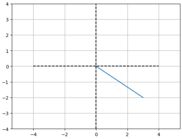
#transposing
v3t = np.transpose(v3)
print(v3t)
# if they're alr numpy arrays you can just v3.T
 
plt.plot([0,v2[0]], [0,v2[1]])
# x coords: [0, v2[0]] = [0, 3], meaning the x-axis starts at 0 and goes to 3
# y coordinates: [0, v2[1]] = [0, -2], meaning the y-axis starts at 0 and goes to -2
# This effectively draws a line from the origin [0, 0] to the point [3, -2]
 
""" === remaining things to make the graph look pretty === """
# ensures the x and y scares are equal
plt.axis('equal') 
# plotting x = -4 to x = 4, k = black, -- = dashed
plt.plot([-4,4],[0,0],'k--')
# plotting y = -4 to y = 4
plt.plot([0,0],[-4,4],'k--')
plt.grid()
# Sets the axis limits so that the x and y range from -4 to 4 (first 2 - x, last 2 - y)
plt.axis((-4,4,-4,4))
plt.show()

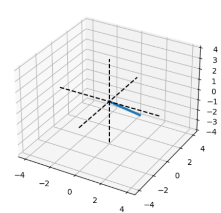
# plotting the 3D vector
fig = plt.figure(figsize=plt.figaspect(1))
ax = fig.add_subplot(111, projection='3d')
ax.plot([0,v3[0]],[0,v3[1]],[0,v3[2]], linewidth=3)
 
# making the plot look nicer
ax.plot([0,0],[0,0],[-4,4],'k--')
ax.plot([0,0],[-4,4],[0,0],'k--')
ax.plot([-4,4],[0,0],[0,0],'k--')

Vector addition and subtraction

v1=np.array([3,-1])
v2=np.array([2,4])
v3 = v1 + v2
 
#plotting them
plt.plot([0,v1[0]],[0,v1[1]], 'b',label='v1')
plt.plot([0,v2[0]] + v1[0],[0,v2[1]] + v1[1], 'r',label='v2')
plt.plot([0,v3[0]],[0,v3[1]],'k',label='v1+v2')
 
plt.legend()
plt.axis('square')
plt.axis((-6,6,-6,6))
plt.grid()
plt.show()

• We want to use numpy arrays because it will broadcast
  • NumPy arrays vs Python lists

Scalar Multiplication

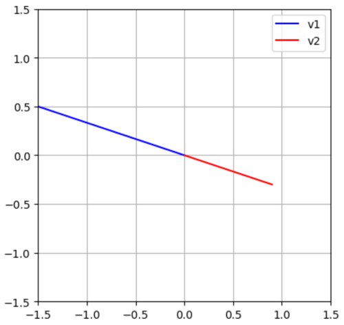
v1 = np.array([-3,1])
l = -0.3
v2 = v1 * l
 
plt.plot([0,v1[0]], [0,v1[1]], 'b', label='v1')
plt.plot([0,v2[0]], [0,v2[1]], 'r', label='v2')
 
plt.axis('square')
# getting whatever is the largest from the elems in the vectors and * 1.5
axlim = max([abs(max(v1)), abs(max(v2))]) * 1.5 
print(axlim)
plt.axis((-axlim, axlim, -axlim, axlim))
plt.grid()
plt.legend();

Vector multiplication

Dot product

$$\begin{array}{rl}{a}^{T}b& =\sum _{i=1}^D{a}_i{b}_i\\ & =||a||||b||\cos ({\theta }_{ab})\\ \text{cos}{\theta }_{ab}& =\frac{a^{T}b}{||a||||b||}\\ {\theta }_{ab}& =\text{arccos}\frac{a^{T}b}{||a||||b||}\\ ||a||& =\sqrt{a^{T}b}\end{array}$$

v1 = np.array([0,4,1,5,3])
v2 = np.array([4,7,8,2,2])
 
"""=== They all do the same thing: dot product ==="""
# method 1
v3 = sum(np.multiply(v1,v2)) # just returning gives a list
print(v3)
 
# method 2
v3 = np.dot(v1,v2)
v3 = v1.dot(v2) # also an instance method
print(v3)
 
# method 3
v3 = np.matmul(v1,v2) # matrix multiplication
print(v3)
 
# method 4
v3 = v1.T @ v2 # "transposing" a 1D aray is the same
v3 = v1 @ v2
print(v3)
 
# method 5 (looping, X rec)
v3 = 0
for i in range(len(v1)):
  v3 += v1[i] * v2[i]
print(v3)
 
# (lazy programmer)
# method 6 =, using zip
dot = 0
a = np.array([1,2])
b = np.array([3.4])
 
for e,f in zip(a,b):
	dot += e * f
print(dot) # 11
 
# multiplying gives us element-wise multiplication
print(a * b) # array([3,8])
print(np.sum(a*b)) # 11
print((a*b).sum()) # 11
 
"""The geometric"""
magnitude_a = np.sqrt(np.dot(a,a)) # or use np.linalg.norm
magnitude_b = np.sqrt(np.dot(b,b))
dot = (magnitude_a * magnitude_b) / np.cos(a,b)
 

• zip in python

Vector magnitude

a = np.random.randn(5)
print(f"a: {a}\n")
 
# 2 ways
magnitude = np.sqrt(np.dot(a,a))
print(f"magnitude: {magnitude}")
 
magnitude = np.linalg.norm(a)
print(f"magnitude: {magnitude}")

Calculating the angle between vectors

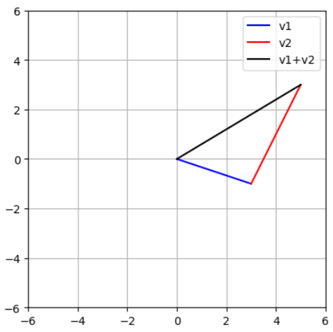
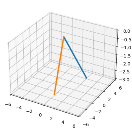
v1 = [2,4,-3]
v2 = [0,-3,-3]
dot_prod = np.dot(v1,v2)
v1_mag = np.linalg.norm(v1)
v2_mag = np.linalg.norm(v2)
theta = np.arccos(dot_prod / (v1_mag * v2_mag))
print(f"theta: {theta} radians") # approximately 90 degrees
 
# plotting the 3D vector
fig = plt.figure()
ax = fig.add_subplot(111, projection='3d')
ax.plot([0,v1[0]],[0,v1[1]],[0,v1[2]], linewidth=3)
ax.plot([0,v2[0]],[0,v2[1]],[0,v2[2]], linewidth=3);
 
plt.axis((-6,6,-6,6)) # only limiting the x and y
plt.show()

Proving the Cauchy-Schwarz inequality

• For dependent vectors (linear combination exist)
  • Equality: $|a^{T}b|=||a||||b||$
• For independent vectors (linear combination doesn’t exist)
  • Inequality: $|a^{T}b|\le ||a||||b||$

# solution in the course
a = np.random.randn(5)
b = np.random.randn(5) # astronomically unlikely they are dependent => b and a are independent vectors!!
c = np.random.randn(1) * a # scalar times a -> c and a are dependent vectors!!
 
dot = np.dot(a,b)
mag_prod = np.linalg.norm(a) * np.linalg.norm(b)
 
# demonstarting inequality |a^T b| <= ||a||||b|| with independent set
print(np.abs(dot) == mag_prod)
print(f"RHS:{np.abs(dot)}")
print(f"LHS:{mag_prod}")
 
# demonstrating equality |a^T b| = ||a||||b|| with dependent set
dot2 = np.dot(a,c)
mag_prod2 = np.linalg.norm(a) * np.linalg.norm(c)
print(np.round(np.abs(dot2),4) == np.round(mag_prod2, 4)) # round to prevent precision error
print(f"RHS:{np.abs(dot2)}")
print(f"LHS:{mag_prod2}")
 
"""Results"""
#False
#RHS:0.18071521267290253
#LHS:2.112102692817962
#True
#RHS:1.4376900820291676
#LHS:1.4376900820291676